cmoroney
Stackoverflow Dataset Analysis
Stackoverflow is the first place any developer goes to in search of solutions for challenges and programming errors that might come up. SO covers the first page of Google results for most if not all common error codes one might throw at it (trust me).
StackOverflow has published a public dataset containing all forum activity between 2008 and 2022. The largest table, questions,
contains over 24 million rows of post content and metadata.
This dataset is accessible via Google BigQuery here: https://cloud.google.com/bigquery/public-data
Note: most EDA performed was done inside GCP and not saved. I did not plan on creating a write up for this until far into the project. I will recreate my EDA process when I have time and update this page.
Problem
Over the years, the userbase has grown quite a bit and as a consequence the number of unanswered questions has grown with it.
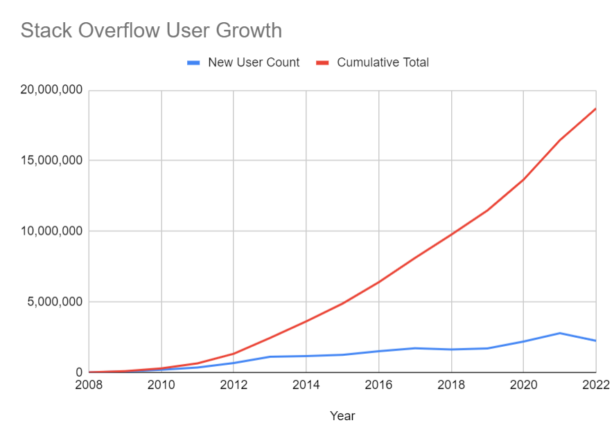
The chart below represents the percentage of questions that have not had any posted answers.

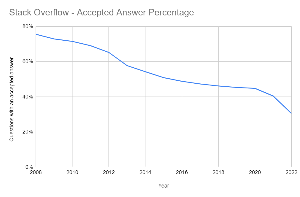
While this paints a picture of the problem, we can dig a little further. Just because someone responds to your question, it doesn’t necessarily mean your question was answered satisfactorily.
Using the same table, we can calculate the percentage of questions with an answer that was accepted by the original asker, suggesting that their question was answered sufficiently.
Business Case
Unanswered questions could lead to a falling user base for Stack Overflow. This could lead to less advertiser interest, and less enterprise business exposure which are two forms of revenue generation at the company currently.
One potential path forward is to identify questions as unanswerable before they are posted. Classifying questions as unanswerable before they are posted may give internal teams at the company an opportunity to intervene - show the user a “answerability” score, offer suggestions to improve the body of their question, suggest better tags, etc.
Data Prep
I will be querying the public dataset from a Jupyter notebook and storing the result in a table in my account for future use.
Question Features
The questions table has a lot of information that you can also see on the post’s corresponding webpage. Features created
from fields in this table:
- Creation date - year, day of week, hour
- Body - this contains html of the post content. HTML and
codetags will be removed to generate text features - Title - character count, question words included
- Total
<code>snippet count <code>snippet length- List tags included in body (boolean)
User Features
The public dataset includes a users table that could provide additional information about the person asking the question.
There is also a table containing badge data. Badges are earned by users for completing different accomplishments. For example, when you ask a question and accept an answer, you will receive a “Scholar” badge.
- Total question badges
- Total answer badges
- Total “other” badges
- Total bronze, silver, and gold tag badges
- Number of questions asked
- Cumulative post score
- User tenure - calculated as a day difference between sign-up and the date which the question is asked
- User profile score
Response variable
I will use questions that no not have any accepted answers as a definition of an “unanswered” question. This provides a more accurate response and provides a more balanced dataset to classify - 49% of all questions have no accepted answer vs 14% having no answer at all.
Completed SQL query:
WITH stackoverflow_questions AS (
        SELECT *
        FROM bigquery-public-data.stackoverflow.posts_questions
        TABLESAMPLE SYSTEM (20 PERCENT)
    ),
    -- WITH
    badges AS (
    -- More info at https://stackoverflow.com/help/badges
      SELECT
        date AS earned_date,
        id,
        user_id,
        name,
        CASE
          WHEN LOWER(name) like '%question%' OR
            name IN ('Altruist', 'Benefactor', 'Curious', 'Inquisitive', 'Socratic', 'Investor', 'Promoter', 'Scholar', 'Student')
          THEN 'question'
          WHEN LOWER(name) like '%answer%' or
            name IN ('Enlightened', 'Explainer', 'Refiner', 'Illuminator', 'Generalist', 'Guru', 'Lifejacket', 'Lifeboat', 'Populist', 'Revival', 'Necromancer', 'Self-Learner', 'Teacher', 'Tenacious', 'Unsung Hero')
          THEN 'answer'
          WHEN tag_based AND class = 1 THEN 'gold_tag'
          WHEN tag_based AND class = 2 THEN 'silver_tag'
          WHEN tag_based AND class = 3 THEN 'bronze_tag'
          ELSE 'other_badge'
        END AS badge_type
      FROM bigquery-public-data.stackoverflow.badges
      ORDER BY 2
    ),

    calc_features AS (
    SELECT
      q.id,
      q.creation_date,
      q.owner_user_id,
      q.body,
      q.title,
      regexp_replace(
        regexp_replace(
                    regexp_replace(q.body, r'''<code>(.|\s)*</code>''', ''), r'''<([a-zA-Z\s]|/[a-zA-Z\s])*>''', ''
                ), '''<[^>]+>''', ''''''
            ) as body_text,

      -- Date features
      EXTRACT(year FROM q.creation_date) AS year,
      EXTRACT(dayofweek FROM q.creation_date) AS dow,
      EXTRACT(hour from q.creation_date) AS hour,

      -- Title / body features
       array_to_string(regexp_extract_all(body, r'''<code>([^<]+)<\/code>'''), '''\n''') AS code_text,
      array_length(regexp_extract_all(body, r'''<code>([^<]+)<\/code>''')) AS total_code_snippets,
      length(array_to_string(regexp_extract_all(body, r'''<code>([^<]+)<\/code>'''), '''\n''')) AS code_length,

      length(replace(q.title, ''' ''', '')) AS title_character_count,
      array_length(regexp_extract_all(trim(q.title), ''' ''')) + 1 AS title_word_count,
      array_length(split(trim(regexp_replace(tags, r'''\|''', ',')))) AS total_tags,
      regexp_contains(title, '''^\\b[A-Z][a-z]*\\b''') AS title_init_title_case,
      regexp_contains(title, r'''\\?$''') AS title_term_question,
      regexp_contains(lower(title), '^who|what|when|where|why|how .*$') AS title_init_wh,
      body like '%<ul>%<li>%</li>%</ul>%' AS body_contains_list,

      -- User profile features
      u.about_me IS NOT NULL AS has_about_me,
      u.profile_image_url IS NOT NULL as has_profile_image,
      u.website_url IS NOT NULL AS has_website_url,
      q.score,

      -- User history features
      DATE_DIFF(q.creation_date, u.creation_date, DAY) AS user_tenure,
      COALESCE(
        SUM(q.score) OVER (PARTITION BY q.owner_user_id
          ORDER BY q.creation_date
          ROWS BETWEEN UNBOUNDED PRECEDING AND 1 PRECEDING)
       , 0) AS cummulative_post_score,
      rank() OVER(PARTITION BY q.owner_user_id ORDER BY q.creation_date) AS questions_asked,
      COUNT(CASE WHEN b.badge_type = 'question' THEN b.id END) AS question_badges,
      COUNT(CASE WHEN b.badge_type = 'answer' THEN b.id END) AS answer_badges,
      COUNT(CASE WHEN b.badge_type = 'other_badge' THEN b.id END) AS other_badges,
      COUNT(CASE WHEN b.badge_type = 'bronze_tag' THEN b.id END) AS bronze_tag_badges,
      COUNT(CASE WHEN b.badge_type = 'silver_tag' THEN b.id END) AS silver_tag_badges,
      COUNT(CASE WHEN b.badge_type = 'gold_tag' THEN b.id END) AS gold_tag_badges,

      -- Two options for response variable
      SUM(answer_count) > 0 AS answer_boolean,
      accepted_answer_id IS NOT NULL AS accepted_answer_boolean

    FROM stackoverflow_questions q
    LEFT JOIN badges b
      ON q.owner_user_id = b.user_id
      AND b.earned_date < q.creation_date
    LEFT JOIN `bigquery-public-data.stackoverflow.users` u
      ON q.owner_user_id = u.id
    WHERE q.owner_user_id IS NOT NULL
    GROUP BY 1,2,3,4,5,6,7,8,9,10,11,12,13,14,15,16,17,18,19,20,21,22,23,24,34
    )

    SELECT
      id,
      -- Text features
      body_text,
      title AS title_text,

      -- Categorical features
      year AS year_cat,
      dow AS dow_cat,
      hour AS hour_cat,
      title_init_title_case AS title_case_cat,
      title_term_question AS title_question_cat,
      title_init_wh AS title_w_cat,
      body_contains_list AS body_list_cat,
      has_about_me AS about_me_cat,
      has_profile_image AS profile_image_cat,
      has_website_url AS website_url_cat,

      -- Numeric features
      length(body_text) AS body_length_num,
      total_code_snippets AS code_snippets_num,
      code_length AS code_length_num,
      code_length / nullif(length(body_text), 0) AS code_to_words_num,
      title_character_count AS title_length_num,
      title_word_count AS title_wordcount_num,
      total_tags AS tag_count_num,
      user_tenure AS user_tenure_days_num,
      cummulative_post_score AS cumm_post_score_num,
      questions_asked AS ques_asked_num,
      question_badges AS ques_badges_num,
      answer_badges AS answer_badges_num,
      other_badges AS other_badges_num,
      bronze_tag_badges AS bronze_badges_num,
      silver_tag_badges AS silver_badges_num,
      gold_tag_badges AS gold_badges_num,

      -- Response variable
      answer_boolean,
      accepted_answer_boolean

    FROM calc_features
Additional data prep in Python
Once the data is extracted from BigQuery, we can start to manipulate it in Python to enrich the dataset with more features.
Compress integer columns
Since this query outputs a fairly large dataset (~20 million rows x 37 columns), we will need to make some adjustments along the
way to assure that we can work with it in-memory. First we will compress the int columns as Google BigQuery assigns int64
by default. Since the numeric data in the dataset are smaller integers, we can take advantage of int8, int16, and
int32 data types to shrink the size of our training set.
Function:
def compress_int_columns(data):
    int8_cols = []
    int16_cols = []
    for i in df.columns[data.dtypes == 'int64']:
        if i != "Unnamed: 0":
            col_max = data[i].max()
            # col_min = data[i].min()

            if col_max < 32767:
                if col_max < 127:
                    int8_cols.append(i)
                else:
                    int16_cols.append(i)

    for col in int8_cols:
        data[col] = data[col].astype(np.int8)

    for col in int16_cols:
        data[col] = data[col].astype(np.int16)

    return data
Then we can use this to compress any int64 columns by writing
df = compress_int_columns(df)
Simple text features
We can add a few additional text features by writing a few one-line functions:
def count_chars(str):
    return len(str)

def word_count(str):
    return len(str.split())

def count_unique_words(str):
        return len(set(str.split()))
We can also use more advanced methods from the textstatistics and SpaCy packages:
def syllables_count(text):
        return textstatistics().syllable_count(text)

# Count total number of sentences and difficult words
def add_spacy_features(data):
        sentences_out = []
        diff_words_out = []
        for chunk in np.array_split(data, 10):
            nlp = spacy.load('en_core_web_sm')
            docs = list(nlp.pipe(chunk,
                                 # Disable pipeline processes that won't be used
                                 disable=['toke2vec', 'tagger', 'attribute_ruler', 'lemmatizer', 'ner', 'entity_linker',
                                          'entity_ruler', 'textcat'],
                                 n_process=4
                                 ))

            for doc in docs:
                words = []
                sentences = doc.sents
                for sentence in sentences:
                    words += [str(token) for token in sentence]

                diff_words_set = set()

                for word in words:
                    syllable_count = syllables_count(word)
                    if word not in nlp.Defaults.stop_words and syllable_count >= 2:
                        diff_words_set.add(word)

                sentences_out.append(len(list(doc.sents)))
                diff_words_out.append(len(diff_words_set))

        return [sentences_out, diff_words_out]
SpaCy is an expansive natural language processing (NLP) package for Python. I am only scratching the surface of what is capable with in this writeup so I suggest checking out the website for more information.
From the features created using the above functions, we can calculate readability scores:
- Flesch Reading Ease (RE) score =- 206.835 - (1.015 x
ASL) - (84.6 xASW) , whereASL= average sentence length andASW= average syllables per word - Gunning Fog Readability Index = 0.4 x (average sentence length + percentage of difficult words)
Preprocessing
In my original SQL query, I added suffixes to each feature type to make it easier to split them up for preprocessing later. Now I can create arrays of column names for each data type, and create a combined array with all columns to use for X:
df = df.sample(n=10000, random_state=0)

categorical_features = [col for col in df.columns if '_cat' in col]
numeric_features = [col for col in df.columns if '_num' in col]
text_features = ['body_text']

all_features = text_features  + categorical_features + numeric_features

X = df[all_features]
y =df["accepted_answer_boolean"].astype('int')
For categorical features, I am using a one-hot encoding transformation for simplicity. There are other (potentially better performing) methods for some of these features that are worth testing. For instance, time features like hour of day or day of week can be sine/cosine transformed to retain the cyclical nature.
categorical_preprocessing = Pipeline([
    ('One Hot Encoding', OneHotEncoder(handle_unknown='ignore'))
])
For numerical features, StandardScaler() is used to remove the mean from each observation and scale to unit variance. See
Sklearn preprocessing methods for more info.
numeric_preprocessing = Pipeline([
    ('scaling', StandardScaler())
])
Base Model
Let’s fit a base model using only the numeric and categorical features to get an idea of predictive accuracy before adding more complex NLP features.
To choose the best algorithm for this classification task I will use GridSearchCV() with several classifiers and
a small subset of the data. The grid search will train each model with randomized hyperparameters, providing accuracy scores for each model
and hyperparameter subset. After choosing the best performing algorithm, I will do a more thorough parameter search on a much larger
sample for a final model.

I will test several estimators for various reasons:
- Logistic regression as a simpler, more interpretable candidate
- Support Vector Machines as a memory-efficient and high dimensionality effective candidate
- XGBoost as a robust ensemble method for most tasks (“swiss army knife” of ML)
- LightGBM as an alternative/comparison to XGBoost
Using a grid search, we can train all 4 models by creating an array of dictionaries that we will feed to the CV.
from sklearn.linear_model import LogisticRegression
from sklearn.svm import LinearSVC
import xgboost as xgb
import lightgbm as lgb
from sklearn.feature_selection import VarianceThreshold

search_space = [{'classifier': [LogisticRegression(solver='sag', max_iter=10000, penalty="l2")]},
                {'classifier': [LinearSVC(max_iter=10000, dual=False)]},
                {'classifier': [xgb.XGBClassifier(tree_method='gpu_hist')]},
                {'classifier': [lgb.LGBMClassifier()]},
                ]
Now within our pipeline, a dummy estimator needs to be defined so that when the program gets to the classifier portion the
grid is referenced and each model is trained with preprocessed data. Within the pipeline, each transformer is required to
have fit and transform methods, so in this dummy function we will have those method calls pass to the next section of code.
We then will pass the dummy estimator (which is really a search grid of classifiers) to the final step of the Sklearn pipeline.
from sklearn.base import BaseEstimator
class DummyEstimator(BaseEstimator):
    def fit(self): pass
    def score(self): pass

text_clf = Pipeline([
    ('preprocessing', preprocessor),
    ('vt', VarianceThreshold()),
    ('classifier', DummyEstimator())
])

grid_search = GridSearchCV(text_clf,
                           param_grid=search_space,
                           scoring=['accuracy'],
                           verbose=3, # highest verbosity - a lot of info is printed during training
                           cv=cv,
                           refit=False, # do not refit on the selected model we will be building a new one
                           error_score='raise' # training will stop and raise an error
                           )
Model Fit and Performance
Now that we have a pipeline and search grid defined, we can call model.fit with the training data, then assess model
performance on the object afterwards.
grid_search.fit(X, y)
print(grid_search.cv_results_)
The cv_results_ method outputs a clean table of each grid search combination (in this case 4 classifiers) along with
mean timings and performance. Truncated tables included times and accuracy:
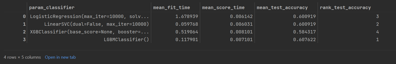
LinearSVC was the fastest classifier for both fit and score timing, and came in second for rank accuracy. LightGBM was the most accurate, with 60.76% mean test accuracy from a 5-fold cross validation.
Although our best performing classifier shows better prediction accuracy than a coin flip, it is still not a very good estimator. Next, we can test some more advanced NLP feature extraction methods to see if our model improves at all.
Text Preprocessing - Vectorization
Vectorization is the general term used for converting a collection of text documents into numerical representations (feature vectors). The simplest form of vectorization is the bag of words model. This model assigns an id to each distinct word in a given corpus (tokenization). Then, each document in the dataset is transformed to an array the size of the vocabulary, with a 1 or 0 in place for each index representing whether the document contains each distinct word. Count vectorizing uses the count of each word in the document rather than a boolean.
Term frequency-inverse document frequency (TF-IDF) goes a step further. This method has two parts:
- TF (term frequency) = (Frequency of a word in a document / Total number of words in that document)
- IDF (inverse document frequency) = log(Total # of documents / documents containing a given word)
The reason behind using the inverse is the idea that the more common a word is across all documents, the less likely it is important for the current document.
Sklearn has a function that combines the CountVectorizer() and TfidfTransformer() pipeline steps into one called
TfidfVectorizer.
Let’s transform the body text field using the TfidfVectorizer() and see what our top words are. The parameter min_df
allows you to adjust the number of features that are returned, according to how many documents each token is present in. I
am setting min_df to 0.01 which tells the transformer to return only tokens that occur in at least 1% of all documents.
tfidf = TfidfVectorizer(stop_words='english', min_df=0.01)
out = tfidf.fit_transform(df['body_text'])
out
<9998x24965 sparse matrix of type '<class 'numpy.float64'>'
	with 253973 stored elements in Compressed Sparse Row format>
So the transformer generated a feature list of 24,965 unique words from the corpus (our ‘body_text’ column).
feature_array = np.array(tfidf.get_feature_names_out())
tfidf_sorting = np.argsort(out.toarray()).flatten()[::-1]

n = 3
top_n = feature_array[tfidf_sorting][:n]
top_n
array(['create', 'image', 'project', 'want', 'custom'], dtype=object)
These are the top 5 most common words in our corpus.
This is what it looks like inside of the pipeline:
from sklearn.feature_extraction.text import TfidfVectorizer
from sklearn.preprocessing import OneHotEncoder, StandardScaler, FunctionTransformer
from sklearn.compose import ColumnTransformer
from sklearn.pipeline import Pipeline

X = df[['body_text']] # Double brackets to keep X as a dataframe instead of a series
y = df['accepted_answer_boolean'].astype('int')

# Combine preprocessing steps to add to pipeline
preprocessor = ColumnTransformer(transformers=[
    # TfidfVectorizer expects a string to be passed, so each text column must be passed in a separate step
    ('text', text_preprocessing, 'body_text'),
])

pipe = Pipeline([
    ('preprocessing', preprocessor),
    ('vt', VarianceThreshold()),
    ('classifier', DummyEstimator())
    ])

cv = KFold(n_splits=5)

grid_search = GridSearchCV(pipe,
                           param_grid=search_space,
                           # scoring=['accuracy'],
                           verbose=3,
                           cv=cv,
                           refit='accuracy',
                           error_score='raise')

print_time('starting...')
grid_search.fit(X, y)
print_time('finished')
I am using these parameter values to decrease training time for the purpose of this project. If time isn’t a factor or RAM is less of a concern, these parameters should be searched and optimized over for prediction performance.
- stop_words - This tells the vectorizer which language to use for stop words. You can choose to leave stop words in, I have taken out English stop words as I know from working with this dataset that keeping them in has no benefit on model accuracy.
- lowercase - Setting
Truewill transform all words to lowercase before processing. This could have implications for part-of-speech tagging, so make sure to test both before deciding. - max_features - Maximum number of feature columns to include in the model. A corpus could contain tens- or hundreds- of thousands of words. I chose to keep the 1000 top features by term frequency in order to avoid memory constraints later on.
- dtype - The feature data output defaults to
float64which has more decimal places and is therefore more accurate thanfloat32but also consumes more memory.
(See Sklearn documentation for full parameter description.)
Checking the results:
pd.DataFrame(grid_search.cv_results_)[['param_classifier',
                                       'mean_fit_time',
                                       'mean_score_time',
                                       'mean_test_accuracy',
                                       'rank_test_accuracy']]
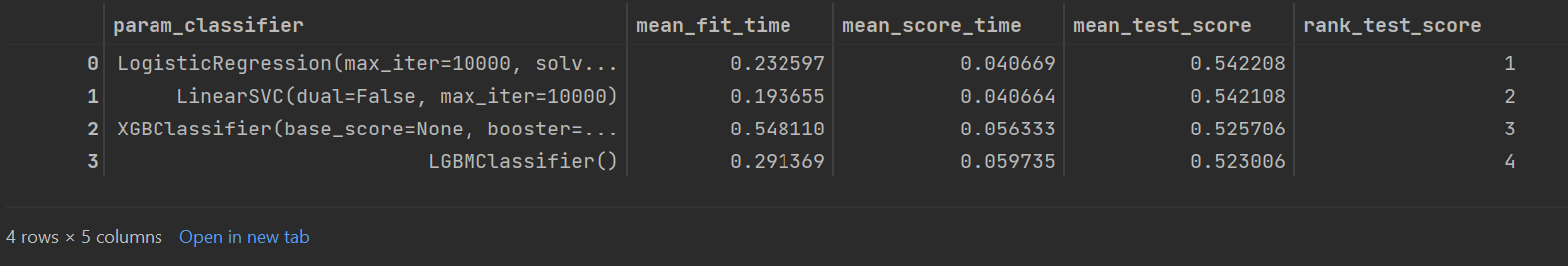
CV Results This time, scores are even lower than the model with only numeric and categorical features. Logistic regression performed the best, although LinearSVC wasn’t far behind.
Tfidf doesn’t seem to bring much to the table in terms of prediction accuracy in this problem.
Word2Vec
While tfidf allows us to quickly generate features based on word frequency across documents, it doesn’t give us any
context around what the words mean within a sentence/document. It also inflates our feature set as similar words are not accounted
for (for example, “written” and “wrote” are similar but are represented as two unique words).
Word2vec is a method patented by Google in 2013 that aims to create word embeddings from neural networks that allow for a deeper machine-readable representation of text. Word2vec allows for comparisons to be made between vector representations of words that actually make sense. One common example of this in use is the king - man + woman = queen example. Put simply, one can argue that if you replace “man” in the definition of the word “king” with “woman”, the logical answer is “queen”. With word2vec, if you use the vectorized representations of all of these words you can show that the two sides are equal. This allows machine learning algorithms to extract more information from text and thus allows for better prediction.
Doc2Vec
Doc2vec is a generalization of word2vec which instead of vectorizing each individual word in a document, a vector is generated for the entire document.
This method may not be very applicable to our problem, as the intuition would be that documents containing similar context should have the same outcome. The issue with our problem is that most questions on StackOverflow have very similar context - I am encountering X error, how can I change my code to fix it?
Another issue I could see is that the same exact error message could have different solutions depending on the system or environment set up. We’ve all been there - you search for an error message you’re frustrated with, try 5 different fixes to no avail. Often times more information is needed in order to adequately solve a problem that comes up.
I will go through implementation of Doc2Vec for demonstration purposes.
First, we need to import libraries and set up a transformer function. We will also create a function that converts text to
lowercase, then runs it through some built-in filters from the gensim package.
from gensim.models.doc2vec import TaggedDocument, Doc2Vec
from sklearn.base import BaseEstimator, TransformerMixin
from sklearn import utils
from tqdm import tqdm
from gensim import utils
import gensim.parsing.preprocessing as gsp
from sklearn import utils as skl_utils

filters = [
           gsp.strip_tags,
           gsp.strip_punctuation,
           gsp.strip_multiple_whitespaces,
           gsp.strip_numeric,
           gsp.remove_stopwords,
           gsp.strip_short,
           gsp.stem_text
          ]

def clean_text(s):
    s = s.lower()
    s = utils.to_unicode(s)
    for f in filters:
        s = f(s)
    return s

class Doc2VecTransformer(BaseEstimator):
    def __init__(self, vector_size=100, learning_rate=0.02, epochs=20):
        self.learning_rate = learning_rate
        self.epochs = epochs
        self._model = None
        self.vector_size = vector_size
        self.workers = 4

    def fit(self, raw_documents, df_y=None):
        tagged_x = [TaggedDocument(clean_text(row).split(), [index]) for index, row in enumerate(raw_documents)]
        model = Doc2Vec(documents=tagged_x, vector_size=self.vector_size, workers=self.workers)
        for epoch in range(self.epochs):
            model.train(skl_utils.shuffle([x for x in tqdm(tagged_x)]), total_examples=len(tagged_x), epochs=1)
            model.alpha -= self.learning_rate
            model.min_alpha = model.alpha

        self._model = model
        return self

    def transform(self, raw_documents):
        return np.asmatrix(np.array([self._model.infer_vector(clean_text(row).split()) for index, row in enumerate(raw_documents)]))
Here’s what a pipeline might look like:
from sklearn.model_selection import RandomizedSearchCV, KFold

df = pd.read_csv('enhanced_output.csv')
df = df.sample(n=10000, random_state=0)
print("dropping NA's...")
df.dropna(inplace=True)

text_preprocessing = Pipeline(steps=[
    ('doc2vec', Doc2VecTransformer())
])

cv = KFold(n_splits = 5)

param_grid = {
              # best params from prior runs
              'classifier__max_depth': [4, 5, 6],
              'classifier__gamma': [0.05, 0.25, 0.5],
              'classifier__colsample_bytree': [0.8, 1.0],
              'classifier__learning_rate': [0.01, 0.05, 0.1],
              'classifier__subsample': [0.2, 0.3, 0.4],
              'preprocessing__text__doc2vec__vector_size':[5, 10, 25],
              'preprocessing__text__doc2vec__learning_rate':[0.01, 0.05, 0.1],
              'preprocessing__text__doc2vec__epochs':[10, 50, 100],
              }

# Combine preprocessing steps to add to pipeline
preprocessor = ColumnTransformer(transformers=[
    ('text', text_preprocessing, 'body_text'),
])

final_text_clf = Pipeline([
    ('preprocessing', preprocessor),
    ('vt', VarianceThreshold()),
    ('classifier', xgb.XGBClassifier(tree_method='gpu_hist',
                                     gpu_id=0))
])

d2v_rs = RandomizedSearchCV(final_text_clf,
                              param_distributions=param_grid,
                              refit=True,
                              cv=cv,
                              verbose=3,
                              n_iter=50,
                              n_jobs=cv.n_splits,
                              error_score='raise',
                              )

print_time("Final model fit begin")
d2v_rs.fit(X, y)
print_time("Final model fit finished")
As suggested, this transformation doesn’t extract meaningful features on this dataset. The best training score I reached was 51% -
not better than a coin flip. I will exclude these features from the final model build and stick with tfidf and our basic
numeric/categorical features.
Training a Final Model
I will try improving our prediction accuracy using a larger portion of the dataset and finer tuning of hyperparameters. Much of the pipeline build will be the same as before, only with a different search space setup and combining feature sets. I am also using XGBoost on the final model as it proved to be more accurate with larger datasets in my previous runs.
We have been using a 10k sample throughout the project, I will increase the sample size to 1 million and do a thorough hyperparameter search for best results.
from sklearn.model_selection import RandomizedSearchCV, KFold

df = pd.read_csv('enhanced_output.csv')
df = df.sample(n=1000000, random_state=0)
print("dropping NA's...")
df.dropna(inplace=True)

categorical_features = [col for col in df.columns if '_cat' in col]
numeric_features = [col for col in df.columns if '_num' in col]
text_features = ['body_text']

all_features = text_features  + categorical_features + numeric_features

X = df[all_features]
y =df["accepted_answer_boolean"].astype('int')

# Set up Kfold cross-validation
cv = KFold(n_splits = 5)

# Create preprocessing steps for each feature type
categorical_preprocessing = Pipeline([
    ('One Hot Encoding', OneHotEncoder(handle_unknown='ignore'))
])

numeric_preprocessing = Pipeline([
    ('scaling', StandardScaler())
])

text_preprocessing = Pipeline(steps=[
    ('squeeze', FunctionTransformer(lambda x: x.squeeze())),
    ('tfidf', TfidfVectorizer(stop_words='english',
                              lowercase=True,
                              max_features=1000, # keep feature size down by limiting building a vocabulary of the top X terms by term frequency
                              dtype=np.float32)), # convert outputs to float32 instead of float64 for memory savings
    ('toarray', FunctionTransformer(lambda x: x.toarray())),
])

param_grid = {
              'classifier__max_depth': [3, 4, 5],
              'classifier__gamma': [0.5, 1, 1.5, 2, 5],
              'classifier__colsample_bytree': [0.6, 0.8, 1.0],
              'classifier__learning_rate': [0.01, 0.02],
              'classifier__subsample': [0.6, 0.8, 1.0]
              }

# Combine preprocessing steps to add to pipeline
preprocessor = ColumnTransformer(transformers=[
    # TfidfVectorizer expects a string to be passed, so each text column must be passed in a separate step
    ('text', text_preprocessing, 'body_text'),
    ('numeric', numeric_preprocessing, numeric_features),
    ('cat', categorical_preprocessing, categorical_features)
])

final_text_clf = Pipeline([
    ('preprocessing', preprocessor),
    ('vt', VarianceThreshold()),
    ('selector', SelectFromModel(estimator=LogisticRegression(max_iter=10000))),
    ('classifier', xgb.XGBClassifier(
        tree_method='gpu_hist',
        gpu_id=0
    )),
])

final_rs = RandomizedSearchCV(final_text_clf,
                              param_distributions=param_grid,
                              refit=False,
                              cv=cv,
                              verbose=3,
                              n_iter=50,
                              n_jobs=cv.n_splits,
                              error_score='raise',
                              )

print_time("Final model fit begin")
final_rs.fit(X, y)
print_time("Final model fit finished")
After nearly 12 hours, the fit finished:
10:33:08 - Final model fit begin
Fitting 5 folds for each of 50 candidates, totalling 250 fits
21:59:55 - Final model fit finished
Now we can pull the best parameters and score using the final_rs object:
print(final_rs.best_params_)
print(final_rs.best_score_)
{'classifier__subsample': 0.6, 'classifier__max_depth': 5, 'classifier__learning_rate': 0.02, 'classifier__gamma': 1.5, 'classifier__colsample_bytree': 0.6}

0.5919286882968179
The score performed better than a 50/50 guess, but not by much at 59.19% accuracy. This was actually slightly worse than the performance from a smaller sample size and using our simple features only.
It is worth noting that a 100x increase in the size of the training data didn’t improve performance, which is a good thing to keep in mind if retraining models for this task going forward.
Conclusion
We tried building a classifier capable of predicting whether or not a user’s question on Stack Overflow would be answered sufficiently
or not. Testing has determined that tfidf and doc2vec are not useful methods for feature extraction in this particular
example, as models trained using the resulting features did rather poorly.
Since the final model did not perform particularly well, it is possible that embeddings are not useful for this problem and that other methods of feature extraction might need to be explored. As it stands, I would consider this project unfeasible if the Stack Overflow team wanted to pursue it as a means of increasing answer rate on questions.
Thank you for reading!
View the full Jupyter Notebook
GitHub Repo: https://github.com/cmoroney/stackoverflow-questions